Chapter 3 clr-lasso
Penalised regression is a powerful approach for variable selection in high dimensional settings (Zou and Hastie 2005; Tibshirani 1996; Le Cessie and Van Houwelingen 1992). It can be adapted to compositional data analysis (CoDA) by previously transforming the compositional data with the centered log-ratio transformation (clr).
Clr-lasso implements penalised regression using the R package glmnet after clr transformation. Clr transformation corresponds to centering the log-transformed values:
\[clr(x) = clr(x_{1},...,x_{k}) = (log(x_{1})-M,...,log(x_{k})-M)\]
Where \(i=1,...,k\) microbial variables, \(x_{k}\) is the counts of variable \(k\), \(M\) is the arithmetic mean of the log-transformed values.
\[M = \frac{1}{k}\sum_{i=1}^{k}log(x_{i})\]
We also generated a wrapper function called glmnet_wrapper() that will help us to handle the output of glmnet. The glmnet_wrapper() function is uploaded via functions.R.
3.1 Crohn case study
First we perform the clr transformation of the abundance table x_Crohn as follows (the log-transformation requires a matrix of positive values and thus the zeros have been previously added with an offset of 1):
z_Crohn <- log(x_Crohn)
clrx_Crohn <- apply(z_Crohn, 2, function(x) x - rowMeans(z_Crohn))
We implement penalised regression with function glmnet(). This function requires the outcome Y to be numeric. The file “Crohn_data.RData” contains y_Crohn_numeric, a numerical vector of disease status with values 1 (CD) and 0 (not CD).
Penalised regression requires the specification of the penalization parameter \(\lambda\). The larger the value of \(\lambda\), the less variables will be selected. In previous analysis of this dataset with selbal, a balance with 12 variables was determined optimal to discriminate the CD status (Rivera-Pinto et al. 2018). For ease of comparison, we will specify the penalisation parameter that results in the selection of 12 variables for clr-lasso.
To identify the value of \(\lambda\) that corresponds to 12 variables selected we implement glmnet() function on the clr transformed values and with the specification that the response family is binomial:
Crohn.test_clrlasso <- glmnet(x = clrx_Crohn, y = y_Crohn_numeric,
                              family = 'binomial', nlambda = 30)
The output of glmnet() can be visualised with the selection plot:
plot(Crohn.test_clrlasso, xvar = 'lambda', label = T)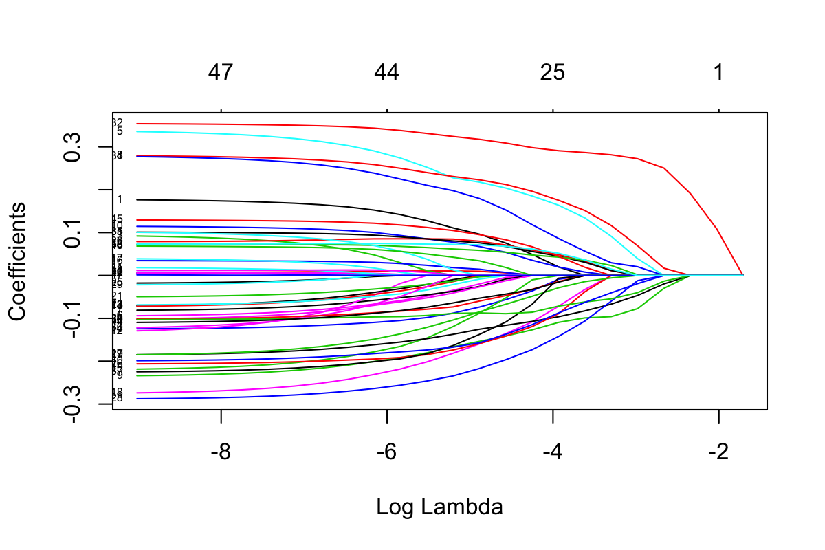
Figure 3.1: Selection plot of Crohn data
In Figure 3.1, each curve corresponds to a variable (i.e. genus). It shows the path of its coefficient against different \(log(\lambda)\) values. At each \(log(\lambda)\), the shown curves indicate the number of nonzero coefficients. In the plot command, if label = T, each curve will be annotated with variable index.
The numerical output of glmnet() will help us to select the value of \(\lambda\). It provides the number of selected variables or degrees of freedom of the model (Df), the proportion of explained deviance for a sequence of values of \(\lambda\):
Crohn.test_clrlasso##
## Call: glmnet(x = clrx_Crohn, y = y_Crohn_numeric, family = "binomial", nlambda = 30)
##
## Df %Dev Lambda
## 1 0 0.00000 0.180900
## 2 1 0.05653 0.131600
## 3 1 0.08761 0.095820
## 4 5 0.12170 0.069750
## 5 10 0.16810 0.050770
## 6 14 0.20670 0.036950
## 7 18 0.24110 0.026900
## 8 23 0.26910 0.019580
## 9 25 0.29220 0.014250
## 10 30 0.30930 0.010370
## 11 32 0.32030 0.007551
## 12 36 0.32770 0.005496
## 13 39 0.33330 0.004001
## 14 41 0.33690 0.002912
## 15 44 0.33910 0.002120
## 16 45 0.34040 0.001543
## 17 46 0.34110 0.001123
## 18 46 0.34150 0.000818
## 19 46 0.34170 0.000595
## 20 47 0.34190 0.000433
## 21 47 0.34190 0.000315
## 22 47 0.34190 0.000230
## 23 47 0.34200 0.000167
## 24 47 0.34200 0.000122We can see that the value of \(\lambda\) that will select 12 variables is between 0.037 and 0.051. We perform again glmnet() with the specification of a finer sequence of \(\lambda\) (between 0.03 and 0.05 and an increment of 0.001):
Crohn.test2_clrlasso <- glmnet(x = clrx_Crohn, y = y_Crohn_numeric,
                               family = 'binomial', lambda = seq(0.03, 0.05, 0.001))
Crohn.test2_clrlasso
##
## Call: glmnet(x = clrx_Crohn, y = y_Crohn_numeric, family = "binomial", lambda = seq(0.03, 0.05, 0.001))
##
## Df %Dev Lambda
## 1 10 0.1702 0.050
## 2 10 0.1729 0.049
## 3 10 0.1755 0.048
## 4 10 0.1782 0.047
## 5 11 0.1808 0.046
## 6 11 0.1834 0.045
## 7 11 0.1860 0.044
## 8 12 0.1885 0.043
## 9 13 0.1915 0.042
## 10 14 0.1945 0.041
## 11 14 0.1976 0.040
## 12 14 0.2006 0.039
## 13 14 0.2036 0.038
## 14 14 0.2065 0.037
## 15 14 0.2094 0.036
## 16 14 0.2122 0.035
## 17 14 0.2150 0.034
## 18 15 0.2181 0.033
## 19 18 0.2217 0.032
## 20 18 0.2257 0.031
## 21 18 0.2295 0.030According to this result, we select \(\lambda = 0.043\) and implement glmnet():
clrlasso_Crohn <- glmnet(x = clrx_Crohn, y = y_Crohn_numeric,
                         family = 'binomial', lambda = 0.043)
The same as selbal, we use function glmnet_wrapper() to handle the results of clr-lasso with the output from glmnet():
Crohn.results_clrlasso <- glmnet_wrapper(clrlasso_Crohn, X = clrx_Crohn)We can get the number of selected variables:
Crohn.results_clrlasso$numVarSelect## [1] 12and the names of the selected variables:
Crohn.results_clrlasso$varSelect## [1] "g__Roseburia" "g__Bacteroides"
## [3] "g__Eggerthella" "f__Peptostreptococcaceae_g__"
## [5] "g__Dialister" "g__Streptococcus"
## [7] "g__Adlercreutzia" "g__Aggregatibacter"
## [9] "o__Clostridiales_g__" "g__Lachnospira"
## [11] "o__Lactobacillales_g__" "g__Bilophila"3.2 HFHS-Day1 case study
The analysis on HFHSday1 data is similar to Crohn data. We first perform the clr transformation:
z_HFHSday1 <- log(x_HFHSday1)
clrx_HFHSday1 <- apply(z_HFHSday1, 2, function(x) x-rowMeans(z_HFHSday1))
The outcome y_HFHSday1 is converted to a numeric vector.
y_HFHSday1_numeric <- as.numeric(y_HFHSday1)We implement glmnet() and visualise the results (Figure 3.2).
HFHS.test_clrlasso <- glmnet(x = clrx_HFHSday1, y = y_HFHSday1_numeric,
family = 'binomial', nlambda = 30)plot(HFHS.test_clrlasso, xvar = 'lambda', label = T)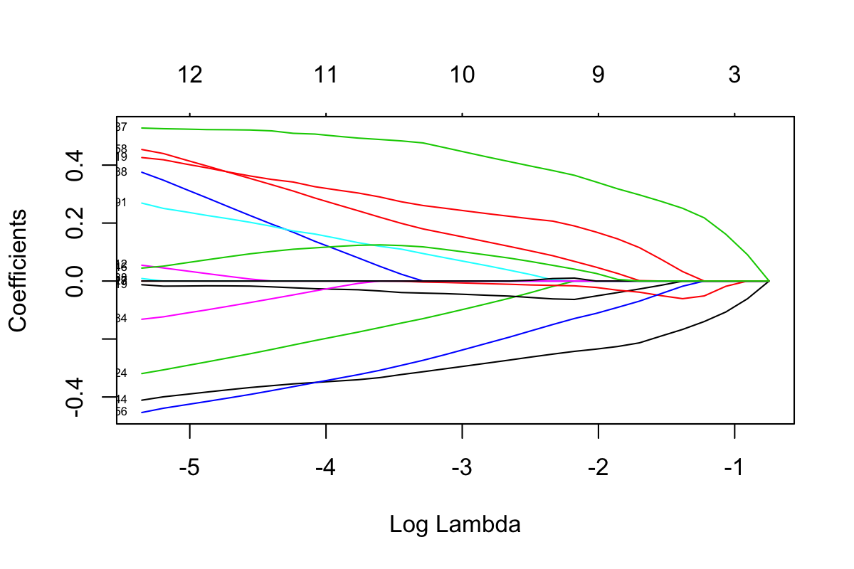
Figure 3.2: Lasso plot of HFHSday1 data
The explanation of Figure 3.2 is the same as Figure 3.1.
The numerical output of glmnet() will help us to decide the penalty term \(\lambda\):
HFHS.test_clrlasso##
## Call: glmnet(x = clrx_HFHSday1, y = y_HFHSday1_numeric, family = "binomial", nlambda = 30)
##
## Df %Dev Lambda
## 1 0 0.0000 0.47370
## 2 2 0.1862 0.40420
## 3 3 0.3290 0.34480
## 4 3 0.4417 0.29420
## 5 6 0.5335 0.25100
## 6 6 0.6089 0.21410
## 7 7 0.6707 0.18270
## 8 8 0.7221 0.15590
## 9 9 0.7649 0.13300
## 10 9 0.8007 0.11350
## 11 11 0.8309 0.09680
## 12 11 0.8564 0.08259
## 13 10 0.8778 0.07046
## 14 10 0.8959 0.06011
## 15 10 0.9113 0.05129
## 16 10 0.9244 0.04376
## 17 10 0.9354 0.03733
## 18 11 0.9449 0.03185
## 19 10 0.9530 0.02717
## 20 11 0.9599 0.02318
## 21 11 0.9657 0.01978
## 22 11 0.9707 0.01688
## 23 11 0.9750 0.01440
## 24 12 0.9786 0.01228
## 25 12 0.9818 0.01048
## 26 12 0.9844 0.00894
## 27 12 0.9867 0.00763
## 28 12 0.9886 0.00651
## 29 12 0.9903 0.00555
## 30 13 0.9917 0.00474For comparison purposes we set the penalty term \(\lambda\) equal to 0.03 (lambda = 0.03) that results in the selection of 10 OTUs.
clrlasso_HFHSday1 <- glmnet(x = clrx_HFHSday1, y = y_HFHSday1_numeric,
                         family = 'binomial', lambda = 0.03)
We then use function glmnet_wrapper() to handle the results:
HFHS.results_clrlasso <- glmnet_wrapper(result = clrlasso_HFHSday1, X = clrx_HFHSday1) Then we get the number of selected variables:
HFHS.results_clrlasso$numVarSelect## [1] 10and the names of selected variables:
HFHS.results_clrlasso$varSelect## [1] "400599" "192222" "348038" "401384" "290253" "261265" "300851"
## [8] "462764" "1108745" "265322"We also extract the taxonomic information of these selected OTUs.
HFHS.tax_clrlasso <- taxonomy_HFHS[which(rownames(taxonomy_HFHS) %in%
                                           HFHS.results_clrlasso$varSelect), ]
kable(HFHS.tax_clrlasso[ ,2:6], booktabs = T)| Phylum | Class | Order | Family | Genus | |
|---|---|---|---|---|---|
| 192222 | Bacteroidetes | Bacteroidia | Bacteroidales | Prevotellaceae | |
| 290253 | Firmicutes | Clostridia | Clostridiales | Ruminococcaceae | Oscillospira |
| 261265 | Firmicutes | Clostridia | Clostridiales | Lachnospiraceae | |
| 1108745 | Firmicutes | Clostridia | Clostridiales | [Mogibacteriaceae] | |
| 462764 | Firmicutes | Clostridia | Clostridiales | Ruminococcaceae | Ruminococcus |
| 265322 | Bacteroidetes | Bacteroidia | Bacteroidales | S24-7 | |
| 400599 | Firmicutes | Clostridia | Clostridiales | ||
| 348038 | Bacteroidetes | Bacteroidia | Bacteroidales | S24-7 | |
| 401384 | Firmicutes | Clostridia | Clostridiales | Ruminococcaceae | Oscillospira |
| 300851 | Firmicutes | Clostridia | Clostridiales | Ruminococcaceae | Oscillospira |
References
Le Cessie, Saskia, and Johannes C Van Houwelingen. 1992. “Ridge Estimators in Logistic Regression.” Journal of the Royal Statistical Society: Series C (Applied Statistics) 41 (1). Wiley Online Library: 191–201.
Rivera-Pinto, J, JJ Egozcue, Vera Pawlowsky-Glahn, Raul Paredes, Marc Noguera-Julian, and ML Calle. 2018. “Balances: A New Perspective for Microbiome Analysis.” MSystems 3 (4). Am Soc Microbiol: e00053–18.
Tibshirani, Robert. 1996. “Regression Shrinkage and Selection via the Lasso.” Journal of the Royal Statistical Society: Series B (Methodological) 58 (1). Wiley Online Library: 267–88.
Zou, Hui, and Trevor Hastie. 2005. “Regularization and Variable Selection via the Elastic Net.” Journal of the Royal Statistical Society: Series B (Statistical Methodology) 67 (2). Wiley Online Library: 301–20.